38 adding labels to graphs in excel
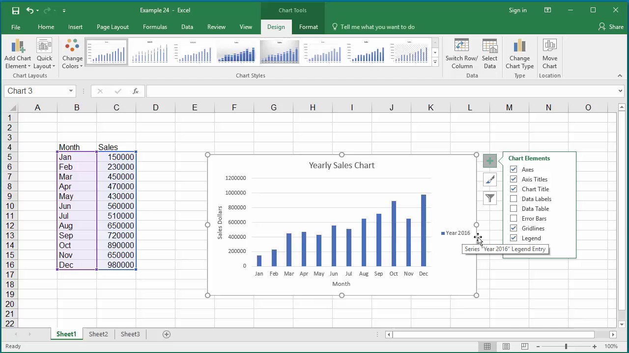
Video: Create a chart On the Recommended Charts tab, scroll through the list of charts that Excel recommends for your data, and click any chart to see how your data will look. If you don’t see a chart you like, click All Charts to see all the available chart types. When you find the chart you like, click it > OK. Use the Chart Elements, Chart Styles, and Chart Filters buttons, next to the upper-right corner of ... How to Add Data Labels to an Excel 2010 Chart - dummies Select where you want the data label to be placed. Data labels added to a chart with a placement of Outside End. On the Chart Tools Layout tab, click Data Labels→More Data Label Options. The Format Data Labels dialog box appears.
› vba › charts-graphsVBA Guide For Charts and Graphs - Automate Excel You can add data labels using the Chart.SetElement method. The following code adds data labels to the inside end of the chart: Sub AddingADataLabels() ActiveChart.SetElement msoElementDataLabelInsideEnd End Sub. The result is: You can specify how the data labels are positioned in the following ways: msoElementDataLabelShow – display data labels.

Adding labels to graphs in excel
How to Add Axis Labels in Excel Charts - Step-by-Step (2022) - Spreadsheeto How to add axis titles 1. Left-click the Excel chart. 2. Click the plus button in the upper right corner of the chart. 3. Click Axis Titles to put a checkmark in the axis title checkbox. This will display axis titles. 4. Click the added axis title text box to write your axis label. Adding Labels to Column Charts | Online Excel Training | Kubicle To add data labels, just right-click on a data series and click add data labels. To see the data labels clearly, I'll need to select them and change their color to white. The data labels are determined by the vertical axis of your chart. Currently, the vertical axis shows millions, therefore, my data labels are shown in millions as well. How to Add Two Data Labels in Excel Chart (with Easy Steps) Table of Contents hide. Download Practice Workbook. 4 Quick Steps to Add Two Data Labels in Excel Chart. Step 1: Create a Chart to Represent Data. Step 2: Add 1st Data Label in Excel Chart. Step 3: Apply 2nd Data Label in Excel Chart. Step 4: Format Data Labels to Show Two Data Labels. Things to Remember.
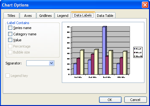
Adding labels to graphs in excel. Data Labels in Excel Pivot Chart (Detailed Analysis) Next open Format Data Labels by pressing the More options in the Data Labels. Then on the side panel, click on the Value From Cells. Next, in the dialog box, Select D5:D11, and click OK. Right after clicking OK, you will notice that there are percentage signs showing on top of the columns. 4. Changing Appearance of Pivot Chart Labels Add data labels and callouts to charts in Excel 365 - EasyTweaks.com The steps that I will share in this guide apply to Excel 2021 / 2019 / 2016. Step #1: After generating the chart in Excel, right-click anywhere within the chart and select Add labels . Note that you can also select the very handy option of Adding data Callouts. Labels in excel graphs - Microsoft Community Click the Insert tab, and then click Line, and pick an option from the available line chart styles . With the chart selected, click the Chart Design tab to do any of the following: (Click Add Chart Element to modify details like the title, labels, and the legend. Click Quick Layout to choose from predefined sets of chart elements. Teach-ICT Computer Science - Excel video tutorials If you want to teach or learn GCSE, Key Stage 3 and A level computer science then come over and have a look at what we have. We have tons of free material as well as professional schemes of work for teachers.
Adding Data Labels To An Excel Chart | MyExcelOnline In our example below, I add a Data Label to a column chart and then I format the data label using CTRL+1. I then select to custom format the numbers so it shows the values as thousands by adding a comma , after each zero and then showing the work k by adding "k" Example Custom Number Format: [$$-1004]#,##0 ,"k" ;- [$$-1004]#,##0 ,"k" Edit titles or data labels in a chart - support.microsoft.com On a chart, click one time or two times on the data label that you want to link to a corresponding worksheet cell. The first click selects the data labels for the whole data series, and the second click selects the individual data label. Right-click the data label, and then click Format Data Label or Format Data Labels. Create a chart from start to finish - support.microsoft.com Note: The Excel Workbook Gallery replaces the former Chart Wizard. By default, the Excel Workbook Gallery opens when you open Excel. From the gallery, you can browse templates and create a new workbook based on one of them. If you don't see the Excel Workbook Gallery, on the File menu, click New from Template. How to Add Data Labels in Excel - Excelchat | Excelchat After inserting a chart in Excel 2010 and earlier versions we need to do the followings to add data labels to the chart; Click inside the chart area to display the Chart Tools. Figure 2. Chart Tools Click on Layout tab of the Chart Tools. In Labels group, click on Data Labels and select the position to add labels to the chart. Figure 3.
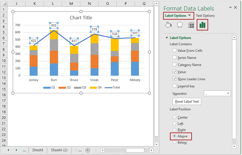
Change the format of data labels in a chart To get there, after adding your data labels, select the data label to format, and then click Chart Elements > Data Labels > More Options. To go to the appropriate area, click one of the four icons ( Fill & Line, Effects, Size & Properties ( Layout & Properties in Outlook or Word), or Label Options) shown here. How to Add X and Y Axis Labels in Excel (2 Easy Methods) 2. Using Excel Chart Element Button to Add Axis Labels. In this second method, we will add the X and Y axis labels in Excel by Chart Element Button. In this case, we will label both the horizontal and vertical axis at the same time. The steps are: Steps: Firstly, select the graph. Secondly, click on the Chart Elements option and press Axis Titles. Find, label and highlight a certain data point in Excel scatter graph Here's how: Click on the highlighted data point to select it. Click the Chart Elements button. Select the Data Labels box and choose where to position the label. By default, Excel shows one numeric value for the label, y value in our case. To display both x and y values, right-click the label, click Format Data Labels…, select the X Value and ... chandoo.org › wp › budget-vs-actual-chart-free-templateFree Budget vs. Actual chart Excel Template - Download May 16, 2018 · Select first line (budget)’s labels and press CTRL+1 to go to format options. Click on “Value from cells” option and point to Var 1 column. Repeat the process for second line (actual) labels too. We get this. Step 13: Adjust label position. We are almost there. Click on the labels and choose position as “Above”.
How to Change Excel Chart Data Labels to Custom Values?
Custom Chart Data Labels In Excel With Formulas - How To Excel At Excel Select the chart label you want to change. In the formula-bar hit = (equals), select the cell reference containing your chart label's data. In this case, the first label is in cell E2. Finally, repeat for all your chart laebls. If you are looking for a way to add custom data labels on your Excel chart, then this blog post is perfect for you.

Custom Data Labels with Colors and Symbols in Excel Charts ...
How to Insert Axis Labels In An Excel Chart | Excelchat We will go to Chart Design and select Add Chart Element Figure 6 - Insert axis labels in Excel In the drop-down menu, we will click on Axis Titles, and subsequently, select Primary vertical Figure 7 - Edit vertical axis labels in Excel Now, we can enter the name we want for the primary vertical axis label.

Microsoft Excel Tutorials: Add Data Labels to a Pie Chart
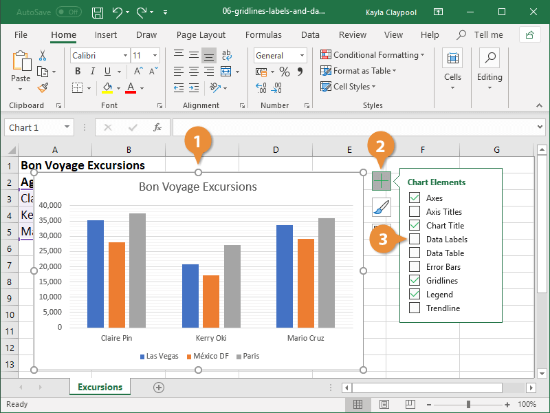
Add or remove data labels in a chart - support.microsoft.com Add data labels to a chart Click the data series or chart. To label one data point, after clicking the series, click that data point. In the upper right corner, next to the chart, click Add Chart Element > Data Labels. To change the location, click the arrow, and choose an option.

Directly Labeling Excel Charts - PolicyViz
How to Place Labels Directly Through Your Line Graph in Microsoft Excel ... Click on Add Data Labels. Your unformatted labels will appear to the right of each data point: Click just once on any of those data labels. You'll see little squares around each data point. Then, right-click on any of those data labels. You'll see a pop-up menu. Select Format Data Labels.

How to Add Total Data Labels to the Excel Stacked Bar Chart ...
How to Add Labels to Scatterplot Points in Excel - Statology Step 3: Add Labels to Points. Next, click anywhere on the chart until a green plus (+) sign appears in the top right corner. Then click Data Labels, then click More Options…. In the Format Data Labels window that appears on the right of the screen, uncheck the box next to Y Value and check the box next to Value From Cells.

Add or remove data labels in a chart
peltiertech.com › broken-y-axis-inBroken Y Axis in an Excel Chart - Peltier Tech Nov 18, 2011 · I did however struggle to get the labels on the x-axis down to the bottom. If I selected the min value of the primary axis for the intercept then the bars in the top primary chart seem to start at the min value of the primary and overwrite the secondary plot. Could you explain how you got he labels to the bottom of the primary axis – thanks ...
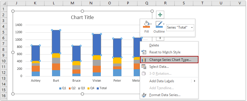
How to add total labels to stacked column chart in Excel?
10 Design Tips to Create Beautiful Excel Charts and Graphs in … 24.09.2015 · To order the graphs in Excel, you'll need to sort the data from largest to smallest. Click 'Data,' choose 'Sort,' and select how you'd like to sort everything. 3) Shorten Y-axis labels. Long Y-axis labels, like large number values, take up a lot of space and can look a little messy, like in the chart below:

Excel Charts: Dynamic Label positioning of line series
› blog › total-labelsHow to add live total labels to graphs and charts in Excel ... Apr 12, 2018 · PowerPoint has a wealth of options for graphs and charts. It offers great ways to display your data visually. For example, a stacked column chart is a way of showing a part-to-whole relationship in the data it represents, whilst also indicating total values of each category.

microsoft excel - How to add comment column as special labels ...
How to Add a Marker Line in Excel Graph (3 Suitable Examples) - ExcelDemy Right-click on the axis and from the side panel, click on the labels Then from the position of the label, select None from the drop-down menu. After some modifications, we got the marker line that will denote the Average value of the Product prices. Read More: How to Make Line Graph in Excel with 2 Variables (With Quick Steps) Conclusion

Add data labels and callouts to charts in Excel 365 ...
Adding rich data labels to charts in Excel 2013 | Microsoft 365 Blog To add a data label in a shape, select the data point of interest, then right-click it to pull up the context menu. Click Add Data Label, then click Add Data Callout . The result is that your data label will appear in a graphical callout. In this case, the category Thr for the particular data label is automatically added to the callout too.

Directly Labeling in Excel
How to Add Two Data Labels in Excel Chart (with Easy Steps) Table of Contents hide. Download Practice Workbook. 4 Quick Steps to Add Two Data Labels in Excel Chart. Step 1: Create a Chart to Represent Data. Step 2: Add 1st Data Label in Excel Chart. Step 3: Apply 2nd Data Label in Excel Chart. Step 4: Format Data Labels to Show Two Data Labels. Things to Remember.

Excel charts: add title, customize chart axis, legend and ...
Adding Labels to Column Charts | Online Excel Training | Kubicle To add data labels, just right-click on a data series and click add data labels. To see the data labels clearly, I'll need to select them and change their color to white. The data labels are determined by the vertical axis of your chart. Currently, the vertical axis shows millions, therefore, my data labels are shown in millions as well.
How to Change Elements of a Chart like Title, Axis Titles, Legend etc in Excel 2016
How to Add Axis Labels in Excel Charts - Step-by-Step (2022) - Spreadsheeto How to add axis titles 1. Left-click the Excel chart. 2. Click the plus button in the upper right corner of the chart. 3. Click Axis Titles to put a checkmark in the axis title checkbox. This will display axis titles. 4. Click the added axis title text box to write your axis label.

Change axis labels in a chart

How to Customize Your Excel Pivot Chart Data Labels - dummies

Dynamically Label Excel Chart Series Lines • My Online ...

Excel Add Axis Label on Mac | WPS Office Academy
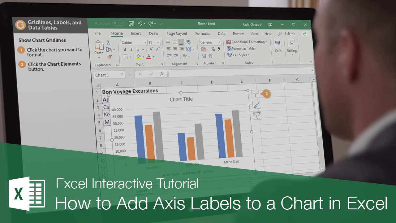
How to Add Axis Labels to a Chart in Excel | CustomGuide

how to add data labels into Excel graphs — storytelling with data

Adding rich data labels to charts in Excel 2013 | Microsoft ...

How to add or move data labels in Excel chart?

Adding rich data labels to charts in Excel 2013 | Microsoft ...

How To Add Axis Labels In Excel - BSUPERIOR

Adding rich data labels to charts in Excel 2013 | Microsoft ...
Adding Data Labels to a Chart (Microsoft Word)

How to Add Two Data Labels in Excel Chart (with Easy Steps ...

How to add total labels to stacked column chart in Excel?

Adding rich data labels to charts in Excel 2013 | Microsoft ...

Excel Add Axis Label on Mac | WPS Office Academy

How to Insert Axis Labels In An Excel Chart | Excelchat

264. How can I make an Excel chart refer to column or row ...
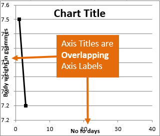
Resize the Plot Area in Excel Chart - Titles and Labels Overlap
How to Add Axis Labels to a Chart in Excel | CustomGuide
How to add total labels to stacked column chart in Excel?

How to label x and y axis in Microsoft excel 2016
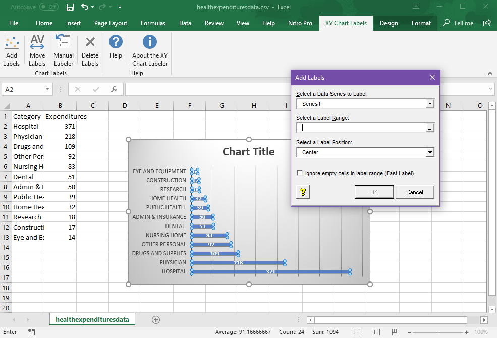
Add Labels to XY Chart Data Points in Excel with XY Chart Labeler

Directly Labeling Your Line Graphs | Depict Data Studio

How to Add Data Labels to an Excel 2010 Chart - dummies
Post a Comment for "38 adding labels to graphs in excel"