45 excel pivot table conditional formatting row labels
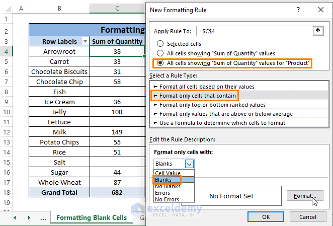
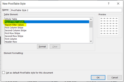
Pivot Table Tips | Exceljet Your pivot table will now use it's own pivot cache and will not refresh with the other pivot table(s) in the workbook, or share the same field grouping. 19. Get rid of useless headings. The default layout for new pivot tables is the Compact layout. This layout will display "Row Labels" and "Column Labels" as headings in the pivot table. Pivot Table Conditional Formatting Based on Another Column ... - ExcelDemy We can conditionally format the entire Pivot Table depending on the blanks. Step 1: Repeat Step 1 of Method 1 then the New Formatting Rule window will open. Here in the New Formatting Rule window, Select the 3rd and 2nd options from Apply Rule to and Select a Rule Type command box respectively. Inside Edit the Rule Description dialog box,
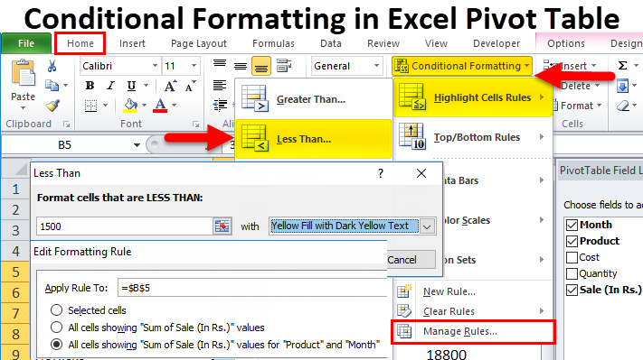
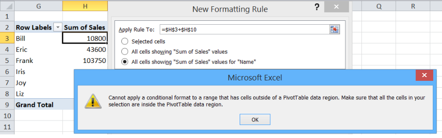
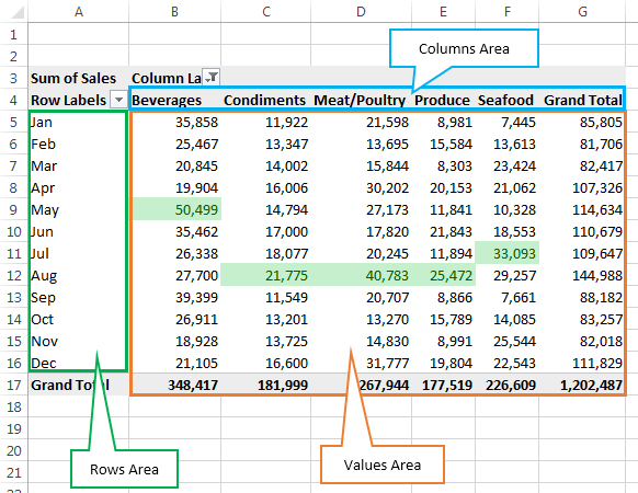
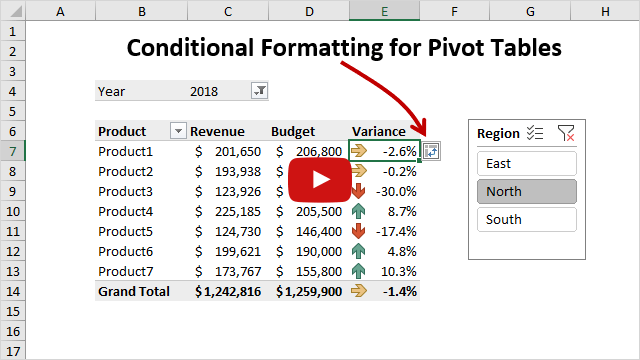
How to Apply Conditional Formatting to Pivot Tables - Excel Campus So in this post I explain how to apply conditional formatting for pivot tables. 1. Select a cell in the Values area The first step is to select a cell in the Values area of the pivot table. If your pivot table has multiple fields in the Values area, select a cell for the field you want to apply the formatting to. 2. Apply Conditional Formatting
Excel pivot table conditional formatting row labels
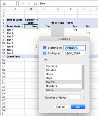
How to Group Numbers in Pivot Table in Excel - Trump Excel You May Also Like the Following Pivot Table Tutorials: How to Group Dates in Pivot Table in Excel. How to Create a Pivot Table in Excel. Preparing Source Data For Pivot Table. How to Refresh Pivot Table in Excel. Using Slicers in Excel Pivot Table – A Beginner’s Guide. How to Apply Conditional Formatting in a Pivot Table in Excel. How to expand all rows in excel pivot table Next, let's check out the pivot table's sheet (named Pivot Table in my example). ). Some of the. Open your spreadsheet in Excel 2013. Click the button above the row 1 heading and to the left of the column A heading to select your entire sheet. Right-click on one of the row numbers, then left-click the Row Height option. Conditional Formatting on Pivot Table row labels As per my knowledge, in this case it does not matter what is the source of pivot as after getting the data in pivot, it's the pivot where the conditional formatting need to be applied, please upload a sample. thanks. Regards, DILIPandey DILIPandey +91 9810929744 dilipandey@gmail.com Register To Reply
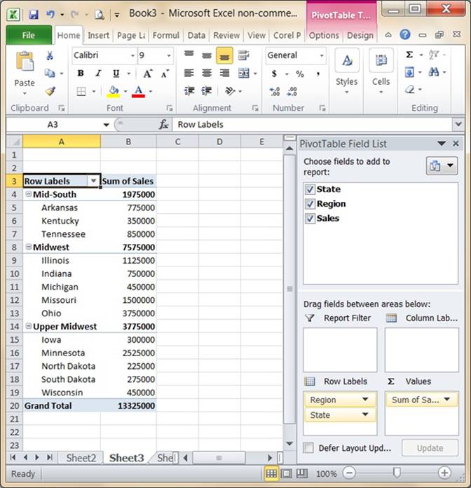
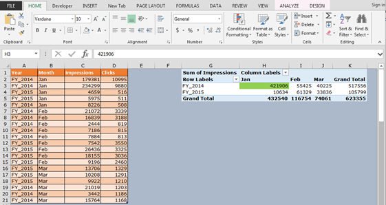
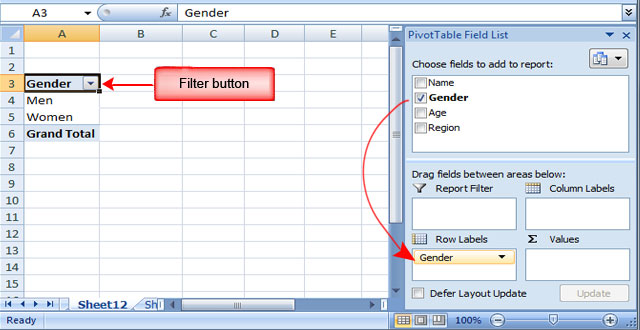
Excel pivot table conditional formatting row labels. How To Compare Multiple Lists of Names with a Pivot Table Jul 08, 2014 · Column E of the Pivot Table contains the Grand Total (sum of columns B:D). People that volunteered all three years will have a “3” in column E. We should sort the pivot table so all the people with a “3” in column E appear at the top … 101 Advanced Pivot Table Tips And Tricks You Need To Know Apr 25, 2022 · Without a table your range reference will look something like above. In this example, if we were to add data past Row 51 or Column I our pivot table would not include it in the results. To create and name your table. Select your data. Go to the Insert tab and press the Table button in the Tables section, or use the keyboard shortcut Ctrl + T. Conditional formatting of Row labels in pivot table I'm looking for a way to set up a condition in a pivot table to output or highlight any row labels that have more than 1 value listed under them. My pivot table has 2 fields listed under Rows. Each of these row labels should only expand with 1 value under them, i want to highlight or output any of the row labels that have more than 1 value listed under them. The Pivot table tools ribbon in Excel These two tabs allow you to perform pivot table customization. This is the Pivot table ribbon in Excel. Create pivot table fields , charts and sets. Here is an important thing to wonder for the pivot table ribbon in excel is as soon as you switch the selected cell to non pivot table cell. The pivot table ribbon disappears.
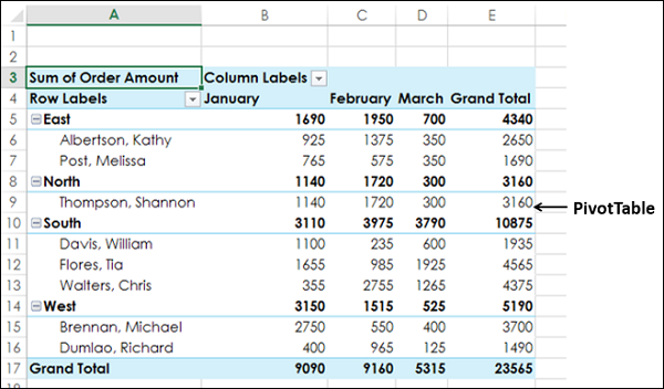
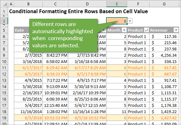
Conditional Formatting in Pivot Table - WallStreetMojo Currently, a pivot table is blank. Next, we need to bring in the values. Then, drag down the "Date" in the "Rows" Label, "Name" in the "Column," and "Sales" in "Values." As a result, the pivot table will look like the one below. To apply conditional formatting in the pivot table, first, we must select the column to format. To create a - uhem.valleymusic.nl Click OK. Once the pivot table sheet is created, just like in the previous example, drag the Category and the Product to the Rows section and the Sales Value to the Values section to get the same Multi-Row pivot table we did in the previous example. Next we want to add a column. Copy conditional Formatting to all rows of Pivot Table Wise people of the forum I have a little question.\. I have a pivot table that has a row of 5 columns with sales results in each. I set up a conditioning format that shows the cells in that row that exceed the average. My question is how do I copy this formatting to all the rows below without having to enter the same formula for each row. Conditional Format Pivot Table Row | Chandoo.org Excel Forums - Become ... I have a pivot table which connects to external data and refreshes on opening. I can conditional format cells based on a value, yet how can I conditional format entire rows based on a cell value? I want to actually hide the referencing column/cell value, but still somehow be able to apply the CF to the entire row. Thanks W
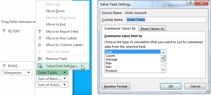
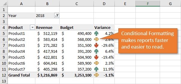
Pivot Table: Pivot table conditional formatting | Exceljet Select any cell in the data you wish to format and then choose "New rule" from the conditional formatting menu on the Home tab of the ribbon. At the top of the window, you will see setting for which cells to apply conditional formatting to. For the example shown, we want: "All cells showing sum of "sales values" for name and "date" Microsoft Excel - Wikipedia Excel 2016 has 484 functions. Of these, 360 existed prior to Excel 2010. Microsoft classifies these functions in 14 categories. Of the 484 current functions, 386 may be called from VBA as methods of the object "WorksheetFunction" and 44 have the same names as VBA functions.. With the introduction of LAMBDA, Excel will become Turing complete.. Macro programming Overwrite pivot table conditional format based on row label As far as I know, using the one rule in the Conditional formatting, we can only format the cells with one color if the condition is true and if the same condition is false, the formatting of the cell will be blank and if both conditions are true, the formatting of cell depends on the highest ranking/priority of the rules in Conditional formatting. 50 Things You Can Do With Excel Pivot Table | MyExcelOnline Jul 18, 2017 · A great way to highlight values within your data set, Excel Table or Pivot Table is to use Conditional Formatting rules. Formatting cells that contain a specific criteria, for example, greater than X or less than X, is a good way to visualize your results. When your criteria references a cell, then you can make this conditional format interactive.
Pivot Table Conditional Formatting Based on Another Column (8 ...
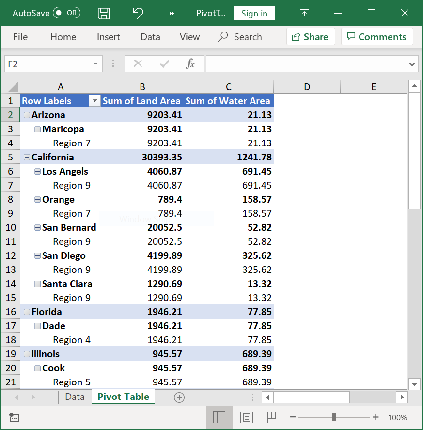
Pivot Table Conditional Formatting for Different Rows Items? Select Your Pivot Table and: Go to Conditional Formatting -> New Rule -> Choose All cells showing "duration" values for "Type and "Date Selection" under "Apply Rule To" section -> Use a Formula to Determine which cells to format and enter the following formula: =AND(A6="Cars",A6>3), You can create new rules for other two conditions as well:
Conditional Formatting in Pivot Table (Example) | How To Apply?
Excel conditional formatting formulas based on another cell - Ablebits.com On the Home tab, in the Styles group, click Conditional formatting > New Rule…; In the New Formatting Rule window, select Use a formula to determine which cells to format.; Enter the formula in the corresponding box. Click the Format… button to choose your custom format.; Switch between the Font, Border and Fill tabs and play with different options such as font style, pattern color and ...
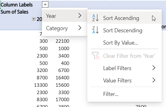
Sort data in a PivotTable or PivotChart
Pivot Table Sort in Excel | How to Sort Pivot Table Columns and … Guide to Pivot Table Sort in Excel. Here we discussed How to Sort Pivot Table Columns and Rows in Excel along with Examples. ... we need to sort the data in the rows so that the Cost Savings column is next to the Row Labels column. To do this, perform the following steps: ... font color, or conditional formatting indicators like sets of icons ...

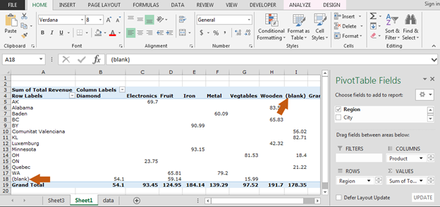
Repeat all item labels in Pivot Table (aka Fill in the blanks ...
Re-Apply Pivot Table Conditional Formatting - yoursumbuddy This method relies on all the conditional formatting you want to re-apply being in that first row labels cell. In cases where the conditional formatting might not apply to the leftmost row label, I've still applied it to that column, but modified the condition to check which column it's in. This function can be modified and called from a ...
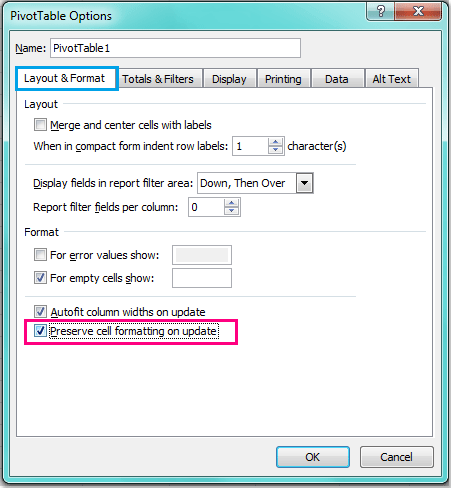
How to preserve formatting after refreshing pivot table?
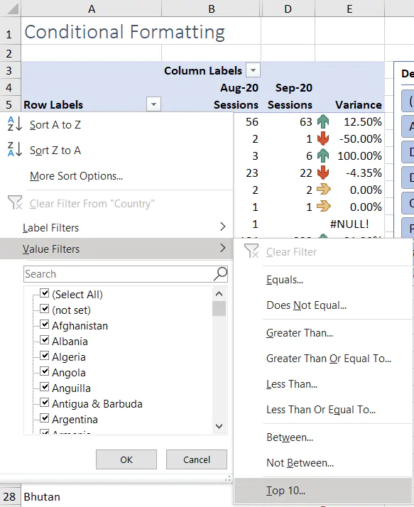
Conditional Formatting in Excel - a Beginner's Guide Here’s what the pivot table looks like when it’s condensed to the top 15 countries. Notice in the image above, the Row Labels and Column Labels header drop downs are missing. For a cleaner look to your pivot table, you can hide your row label and column labels. On the Pivot Table Analyze tab, just click Field Headers to make them disappear ...
Excel PivotTable Percentage: Which Customers Are Costing You ...
Excel VBA: Conditional Format of Pivot Table based on Column Label ... myPivotSourceName = myPivotField.Name. Then rather than referencing the data field with the pivot field object, I referenced the DataRange with the string: myPivotTable.PivotFields (myPivotSourceName).DataRange.Select. Works perfectly and is completely portable for any pivottable on any sheet with any fields. excel vba.
Design the layout and format of a PivotTable
Use Excel with earlier versions of Excel - support.microsoft.com What it means In Excel 97-2007, conditional formatting that contains a data bar rule that uses a negative value is not displayed on the worksheet. However, all conditional formatting rules remain available in the workbook and are applied when the workbook is opened again in Excel 2010 and later, unless the rules were edited in Excel 97-2007.
Dressing Up Your PivotTable Design
Excel pivot table conditional formatting row labels jobs Search for jobs related to Excel pivot table conditional formatting row labels or hire on the world's largest freelancing marketplace with 21m+ jobs. It's free to sign up and bid on jobs.
Excel Pivot Tables - Sorting Data
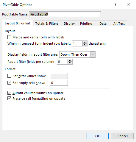
Design the layout and format of a PivotTable To change the layout of a PivotTable, you can change the PivotTable form and the way that fields, columns, rows, subtotals, empty cells and lines are displayed. To change the format of the PivotTable, you can apply a predefined style, banded rows, and conditional formatting. Windows Web Mac Changing the layout form of a PivotTable
Conditional Formatting for Pivot Table
Format Pivot Table Labels Based on Date Range Select all the dates in the Row Labels that you want to format. On the Ribbon, click the Home tab, and then in the Styles group, click Conditional Formatting. In the list of conditional formatting options, click Highlight Cells Rules, and then click A Date Occurring.

Apply Conditional Formatting | Excel Pivot Table Tutorial
Conditional Formatting of Pivot Tables - Excel TV Conditional Formatting of Pivot Tables. Xtreme Pivot Tables. Current Progress. Current Progress. Current Progress 0% Not ... Change SUM Views in Label Areas. Indent Rows in Compact Layouts. Change Layout of a Report Filter. ... New Excel 2013 Pivot Table Features. Cosmetic Changes. Recommended Pivot Tables. Distinct Count. Timeline Slicer.
Working with a Pivot Table that Has Conditional Formatting ...
Formatting Pivot Table Row Labels by Level | MrExcel Message Board hover your cursor over the top line of one of the SubTotals of the Level that you want to format until you get a downward pointing, then left click - that should highlight all the cells at that level right click while hovering over one of the selected cells to format it OR hit Ctrl+F1
Pivot Table Filter | CustomGuide
Pivot table filters - qxmk.bankin.info Skill Level: Intermediate Download the Excel File. Here's the file that I use in the video. You can use it to practice adding, deleting, and changing conditional formatting on a variety of pivot table. Select the sheet with the pivot table and chart, right click on the sheet tab, and choose View Code. This opens the code module for the active ...
Format Pivot Table Labels Based on Date Range | Excel Pivot ...
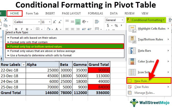
Excel Conditional Formatting in Pivot Table - EDUCBA Click on any cell in the pivot table > Go to the HOME tab > Click on Conditional Formatting option under Styles option > Click on Manage Rules option. It will open a Rules Manager dialog box. Click on the Edit Rule tab, as shown in the below screenshot. It will open the Editing Rule formatting window. Refer to the below screenshot.

How to Apply Conditional Formatting to a Pivot Table in Your ...
Conditional Formatting on Pivot Table row labels As per my knowledge, in this case it does not matter what is the source of pivot as after getting the data in pivot, it's the pivot where the conditional formatting need to be applied, please upload a sample. thanks. Regards, DILIPandey DILIPandey +91 9810929744 dilipandey@gmail.com Register To Reply
Conditional Formatting in Excel - a Beginner's Guide
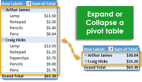
How to expand all rows in excel pivot table Next, let's check out the pivot table's sheet (named Pivot Table in my example). ). Some of the. Open your spreadsheet in Excel 2013. Click the button above the row 1 heading and to the left of the column A heading to select your entire sheet. Right-click on one of the row numbers, then left-click the Row Height option.

How to use Conditional Formatting in the Pivot table ...
How to Group Numbers in Pivot Table in Excel - Trump Excel You May Also Like the Following Pivot Table Tutorials: How to Group Dates in Pivot Table in Excel. How to Create a Pivot Table in Excel. Preparing Source Data For Pivot Table. How to Refresh Pivot Table in Excel. Using Slicers in Excel Pivot Table – A Beginner’s Guide. How to Apply Conditional Formatting in a Pivot Table in Excel.

Pivot Table: Pivot table conditional formatting | Exceljet
How to Remove Blank Rows in Excel Pivot Table (4 Methods ...
How to Apply Conditional Formatting to Pivot Tables - Excel ...
How to Apply Conditional Formatting in Pivot Table? (with ...

How to Apply Conditional Formatting to a Pivot Table in Your ...

How to Apply Conditional Formatting in Pivot Table? (with ...
How to Apply Conditional Formatting to Rows Based on Cell ...
Pivot Table formatting after refresh - Microsoft Community Hub
Lesson 54: Pivot Table Row Labels - Swotster
How to Remove Blanks in a Pivot Table in Excel (6 Ways ...

How to Highlight A row based on Cell Value In Pivot Table ...

Unified Method of Pivot Table Formatting - yoursumbuddy
Conditional Formatting PivotTables • My Online Training Hub
Working with Pivot Tables | Excel library | Syncfusion

Pivot Table Grouping, Ungrouping And Conditional Formatting
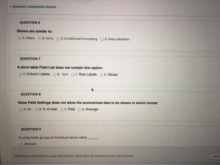
Solved Question Completion Status: QUESTION 6 Slicers are ...
Conditional Formatting in Pivot table
Date Format in Pivot Tables - Microsoft Tech Community
Excel: Apply Conditional Formatting to a Pivot Table - Excel ...

Conditional format a Pivot Table with the wizards ...

Pivot Table Row Labels In the Same Line - Beat Excel!

How to add conditional formatting a Microsoft Excel ...
How to Apply Conditional Formatting to Pivot Tables - Excel ...
101 Advanced Pivot Table Tips And Tricks You Need To Know ...

Conditional format a Pivot Table with the wizards ...

Pivot Table Conditional Formatting

Use an Excel Pivot Table to Count and Sum Values – BatchGeo Blog
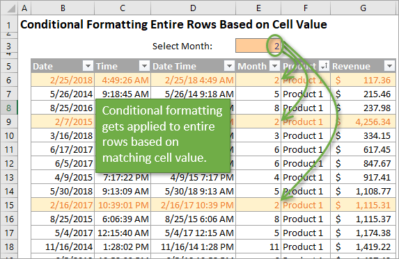
How to Apply Conditional Formatting to Rows Based on Cell ...
Post a Comment for "45 excel pivot table conditional formatting row labels"